使用Tensorflow以图形方式表示MNIST的学习权重

我正在修补关于Tensorflow的教程Deep MNIST for Experts，我试图用图像中的多层卷积网络来表示学习的权重 . 上面的教程有一个更简单的，MNIST For ML Beginners，显示该图像代表训练模型的学习权重 .

This is my code:

from tensorflow.examples.tutorials.mnist import input_data
mnist = input_data.read_data_sets('MNIST_data', one_hot=True)
import matplotlib.pyplot as plt
import numpy as np
import random as ran
import tensorflow as tf

def TRAIN_SIZE(num):
    print ('Total Training Images in Dataset = ' + str(mnist.train.images.shape))
    print ('--------------------------------------------------')
    x_train = mnist.train.images[:num,:]
    print ('x_train Examples Loaded = ' + str(x_train.shape))
    y_train = mnist.train.labels[:num,:]
    print ('y_train Examples Loaded = ' + str(y_train.shape))
    print('')
    return x_train, y_train

def TEST_SIZE(num):
    print ('Total Test Examples in Dataset = ' + str(mnist.test.images.shape))
    print ('--------------------------------------------------')
    x_test = mnist.test.images[:num,:]
    print ('x_test Examples Loaded = ' + str(x_test.shape))
    y_test = mnist.test.labels[:num,:]
    print ('y_test Examples Loaded = ' + str(y_test.shape))
    return x_test, y_test

def display_digit(num):
    print(y_train[num])
    label = y_train[num].argmax(axis=0)
    image = x_train[num].reshape([28,28])
    plt.title('Example: %d  Label: %d' % (num, label))
    plt.imshow(image, cmap=plt.get_cmap('gray_r'))
    plt.show()

def display_mult_flat(start, stop):
    images = x_train[start].reshape([1,784])
    for i in range(start+1,stop):
        images = np.concatenate((images, x_train[i].reshape([1,784])))
    plt.imshow(images, cmap=plt.get_cmap('gray_r'))
    plt.show()

x_train, y_train = TRAIN_SIZE(55000)
display_digit(0)
display_mult_flat(0,400)

sess = tf.InteractiveSession()
x = tf.placeholder(tf.float32, shape=[None, 784])
y_ = tf.placeholder(tf.float32, shape=[None, 10])
W = tf.Variable(tf.zeros([784,10]))
b = tf.Variable(tf.zeros([10]))
y = tf.nn.softmax(tf.matmul(x,W) + b)

cross_entropy = tf.reduce_mean(
    tf.nn.softmax_cross_entropy_with_logits(labels=y_, logits=y))
x_train, y_train = TRAIN_SIZE(5500)
x_test, y_test = TEST_SIZE(10000)
LEARNING_RATE = 0.05
TRAIN_STEPS = 1000

sess.run(tf.global_variables_initializer())

train_step = tf.train.GradientDescentOptimizer(LEARNING_RATE).minimize(cross_entropy)
for _ in range(TRAIN_STEPS):
  batch = mnist.train.next_batch(100)
  train_step.run(feed_dict={x: batch[0], y_: batch[1]})
correct_prediction = tf.equal(tf.argmax(y,1), tf.argmax(y_,1))
accuracy = tf.reduce_mean(tf.cast(correct_prediction, tf.float32))

for i in range(10):
    plt.subplot(2, 5, i+1)
    weight = sess.run(W)[:,i]
    plt.title(i)
    plt.imshow(weight.reshape([28,28]), cmap=plt.get_cmap('seismic'))
    frame1 = plt.gca()
    frame1.axes.get_xaxis().set_visible(False)
    frame1.axes.get_yaxis().set_visible(False) 
plt.show()


def weight_variable(shape):
  initial = tf.truncated_normal(shape, stddev=0.1)
  return tf.Variable(initial)

def bias_variable(shape):
  initial = tf.constant(0.1, shape=shape)
  return tf.Variable(initial)

def conv2d(x, W):
  return tf.nn.conv2d(x, W, strides=[1, 1, 1, 1], padding='SAME')

def max_pool_2x2(x):
  return tf.nn.max_pool(x, ksize=[1, 2, 2, 1],
                        strides=[1, 2, 2, 1], padding='SAME')

# First convolution layeer
W_conv1 = weight_variable([5, 5, 1, 32])
b_conv1 = bias_variable([32])
x_image = tf.reshape(x, [-1,28,28,1])

h_conv1 = tf.nn.relu(conv2d(x_image, W_conv1) + b_conv1)
h_pool1 = max_pool_2x2(h_conv1)

# Second convolution layer
W_conv2 = weight_variable([5, 5, 32, 64])
b_conv2 = bias_variable([64])

h_conv2 = tf.nn.relu(conv2d(h_pool1, W_conv2) + b_conv2)
h_pool2 = max_pool_2x2(h_conv2)

# Densely Connected Layer
W_fc1 = weight_variable([7 * 7 * 64, 1024])
b_fc1 = bias_variable([1024])

h_pool2_flat = tf.reshape(h_pool2, [-1, 7*7*64])
h_fc1 = tf.nn.relu(tf.matmul(h_pool2_flat, W_fc1) + b_fc1)

#Dropout
keep_prob = tf.placeholder(tf.float32)
h_fc1_drop = tf.nn.dropout(h_fc1, keep_prob)

#Readout Layer
W_fc2 = weight_variable([1024, 10])
b_fc2 = bias_variable([10])

y_conv = tf.matmul(h_fc1_drop, W_fc2) + b_fc2

#Evaluating the model
cross_entropy = tf.reduce_mean(
    tf.nn.softmax_cross_entropy_with_logits(labels=y_, logits=y_conv))
train_step = tf.train.AdamOptimizer(1e-4).minimize(cross_entropy)
correct_prediction = tf.equal(tf.argmax(y_conv,1), tf.argmax(y_,1))
accuracy = tf.reduce_mean(tf.cast(correct_prediction, tf.float32))
sess.run(tf.global_variables_initializer())

for i in range(20000):
  batch = mnist.train.next_batch(50)
  if i%100 == 0:
    train_accuracy = accuracy.eval(feed_dict={
        x:batch[0], y_: batch[1], keep_prob: 1.0})
    print("step %d, training accuracy %g"%(i, train_accuracy))
  train_step.run(feed_dict={x: batch[0], y_: batch[1], keep_prob: 0.5})

print("test accuracy %g"%accuracy.eval(feed_dict={
    x: mnist.test.images, y_: mnist.test.labels, keep_prob: 1.0}))

for i in range(10):
    plt.subplot(2, 5, i+1)
    weight = sess.run(W_fc2)[:,i]
    plt.title(i)
    plt.imshow(weight.reshape([32,32]), cmap=plt.get_cmap('seismic'))
    frame1 = plt.gca()
    frame1.axes.get_xaxis().set_visible(False)
    frame1.axes.get_yaxis().set_visible(False) 
plt.show()

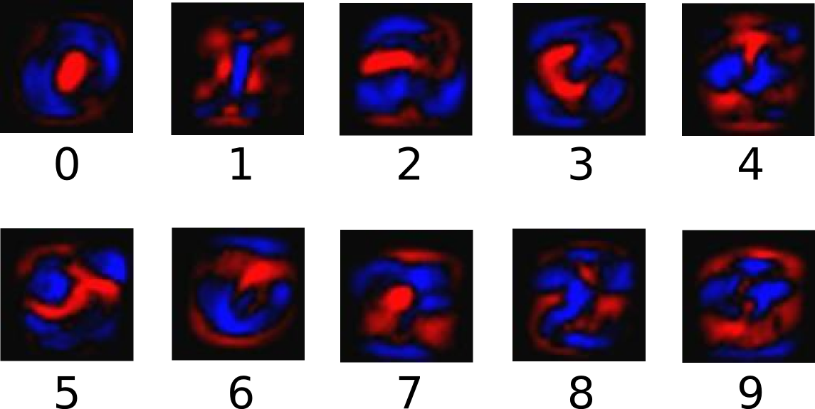
我在 two times 打印学习重量的图像 . 一次作为教程MNIST For ML Beginners中所示的简单MNIST算法的输出，第二次使用多层卷积网络 . The 1st output is correct ：

但是， The 2nd output 使用教程Deep MNIST for Experts中显示的多层卷积网络是：

How do I get the 2nd diagram right?